Backtesting.py 사용법2
backtesting.py -2
백테스팅 라이브러리인 backtesting.py에 대한 유투브 강의 기록.
총 2~8가지의 챕터로 구성 1번 챕터는 별도로 업로드
2. backtest your dollar cost average strategy
https://www.youtube.com/watch?v=Kgr8JjWX0zk&list=PLnSVMZC68_e48lA4aRYL1yHYZ9nEq9AiH&index=2&ab_channel=ChadThackray
- 매수 조건 : 매주 화요일마다 한달 전보다 5% 가격이 하락한 경우
- 매수량 : ‘10’이란 단위를 정해둠. 종가에 따라 share수를 다르게
import pandas as pd
from backtesting import Backtest, Strategy
from backtesting.test import GOOG
import math

class DCA(Strategy):

    amount_to_invest = 10
    def init(self):

        self.day_of_week = self.I(
                                lambda x:x,
                                self.data.Close.s.index.dayofweek,
                                plot=False
                                )

    def next(self):

        if self.day_of_week[-1] == 1 : #every tuesday
            self.buy(size=math.floor(self.amount_to_invest / self.data.Close[-1]))
            try:
                if self.data.Close[-1]/self.data.Close[-30] < 0.95:
                    self.buy(size=math.floor(self.amount_to_invest / self.data.Close[-1]))
            except:
                pass


display(GOOG)
GOOG = GOOG * 10**-6

bt = Backtest(
            GOOG,
            DCA,
            trade_on_close=True,)
stats = bt.run()
display(stats)
bt.plot()
trades = stats['_trades']
price_paid = trades['Size'] * trades['EntryPrice']
total_invested = price_paid.sum()

current_shares = trades['Size'].sum()
current_equity = current_shares * GOOG.Close.iloc[-1]

print("Total investment:", total_invested)
print("Current shares:", current_shares)
print("Current equity:", current_equity)
print("Returns:", (current_equity/total_invested)-1)
print('-'*50)
display(trades)
| Open | High | Low | Close | Volume | |
|---|---|---|---|---|---|
| 2004-08-19 | 100.00 | 104.06 | 95.96 | 100.34 | 22351900 |
| 2004-08-20 | 101.01 | 109.08 | 100.50 | 108.31 | 11428600 |
| 2004-08-23 | 110.75 | 113.48 | 109.05 | 109.40 | 9137200 |
| 2004-08-24 | 111.24 | 111.60 | 103.57 | 104.87 | 7631300 |
| 2004-08-25 | 104.96 | 108.00 | 103.88 | 106.00 | 4598900 |
| ... | ... | ... | ... | ... | ... |
| 2013-02-25 | 802.30 | 808.41 | 790.49 | 790.77 | 2303900 |
| 2013-02-26 | 795.00 | 795.95 | 784.40 | 790.13 | 2202500 |
| 2013-02-27 | 794.80 | 804.75 | 791.11 | 799.78 | 2026100 |
| 2013-02-28 | 801.10 | 806.99 | 801.03 | 801.20 | 2265800 |
| 2013-03-01 | 797.80 | 807.14 | 796.15 | 806.19 | 2175400 |
2148 rows × 5 columns
Start                     2004-08-19 00:00:00
End                       2013-03-01 00:00:00
Duration                   3116 days 00:00:00
Exposure Time [%]                    99.81378
Equity Final [$]                 15291.938059
Equity Peak [$]                  15368.252542
Return [%]                          52.919381
Buy & Hold Return [%]              703.458242
Return (Ann.) [%]                     5.10923
Volatility (Ann.) [%]               12.158924
Sharpe Ratio                         0.420204
Sortino Ratio                        0.639353
Calmar Ratio                         0.187276
Max. Drawdown [%]                  -27.281891
Avg. Drawdown [%]                   -1.522278
Max. Drawdown Duration     1094 days 00:00:00
Avg. Drawdown Duration       45 days 00:00:00
# Trades                                  556
Win Rate [%]                        99.820144
Best Trade [%]                     688.737941
Worst Trade [%]                     -0.700254
Avg. Trade [%]                      79.947572
Max. Trade Duration        3110 days 00:00:00
Avg. Trade Duration        1543 days 00:00:00
Profit Factor                    75574.058032
Expectancy [%]                      95.180471
SQN                                 22.806857
_strategy                                 DCA
_equity_curve                             ...
_trades                         Size  Entr...
dtype: object

Total investment: 5559.868070299999
Current shares: 13544441
Current equity: 10919.39288979
Returns: 0.9639661861977982
--------------------------------------------------
| Size | EntryBar | ExitBar | EntryPrice | ExitPrice | PnL | ReturnPct | EntryTime | ExitTime | Duration | |
|---|---|---|---|---|---|---|---|---|---|---|
| 0 | 12656 | 2144 | 2146 | 0.000790 | 0.000801 | 0.140102 | 0.014010 | 2013-02-26 | 2013-02-28 | 2 days |
| 1 | 12393 | 2139 | 2146 | 0.000807 | 0.000801 | -0.070020 | -0.007003 | 2013-02-19 | 2013-02-28 | 9 days |
| 2 | 12809 | 2135 | 2146 | 0.000781 | 0.000801 | 0.262584 | 0.026258 | 2013-02-12 | 2013-02-28 | 16 days |
| 3 | 13059 | 2130 | 2146 | 0.000766 | 0.000801 | 0.463072 | 0.046308 | 2013-02-05 | 2013-02-28 | 23 days |
| 4 | 13268 | 2125 | 2146 | 0.000754 | 0.000801 | 0.630495 | 0.063051 | 2013-01-29 | 2013-02-28 | 30 days |
| ... | ... | ... | ... | ... | ... | ... | ... | ... | ... | ... |
| 551 | 84860 | 22 | 2146 | 0.000118 | 0.000801 | 57.989930 | 5.799050 | 2004-09-21 | 2013-02-28 | 3082 days |
| 552 | 89694 | 17 | 2146 | 0.000111 | 0.000801 | 61.862849 | 6.186295 | 2004-09-14 | 2013-02-28 | 3089 days |
| 553 | 98444 | 12 | 2146 | 0.000102 | 0.000801 | 68.873391 | 6.887379 | 2004-09-07 | 2013-02-28 | 3096 days |
| 554 | 97684 | 8 | 2146 | 0.000102 | 0.000801 | 68.264510 | 6.826512 | 2004-08-31 | 2013-02-28 | 3103 days |
| 555 | 95356 | 3 | 2146 | 0.000105 | 0.000801 | 66.399243 | 6.639935 | 2004-08-24 | 2013-02-28 | 3110 days |
556 rows × 10 columns
3. Custom Indicators In Backtesting.py - Python Deep Dive
https://www.youtube.com/watch?v=xljQpeYQYkI&list=PLnSVMZC68_e48lA4aRYL1yHYZ9nEq9AiH&index=3&ab_channel=ChadThackray
백테스트를 위한 지표(시그널)을 입력하는 3가지 방법을 다룸
-
데이터에 시그널이 포함되어 있는 경우
-
외부 라이브러리(ex : TA)에서 지표를 계산하는 경우
-
파이썬으로 직접 계산하는 경우
1. Bringing Signal
엑셀이나 파이썬으로 직접 데이터에 시그널을 주고서 하는 방식
- 랜덤으로 정한 시그널로 매수/매도
import pandas as pd
from backtesting import Backtest, Strategy
from backtesting.test import GOOG
import math
import numpy as np

# outside signal
GOOG['Signal'] = np.random.randint(-1, 2, len(GOOG))

class SignalStrategy(Strategy):

    def init(self):
        pass

    def next(self):
        current_signal = self.data.Signal[-1]

        if current_signal == 1:
            if not self.position:
                self.buy()
        elif current_signal == -1:
            if self.position:
                self.position.close()


bt = Backtest(GOOG, SignalStrategy, cash = 10_000)

stats = bt.run()
display(stats)
bt.plot()
Start                     2004-08-19 00:00:00
End                       2013-03-01 00:00:00
Duration                   3116 days 00:00:00
Exposure Time [%]                   69.180633
Equity Final [$]                     26655.53
Equity Peak [$]                      26655.53
Return [%]                           166.5553
Buy & Hold Return [%]              703.458242
Return (Ann.) [%]                   12.189627
Volatility (Ann.) [%]               27.921745
Sharpe Ratio                         0.436564
Sortino Ratio                        0.764974
Calmar Ratio                         0.353457
Max. Drawdown [%]                  -34.486849
Avg. Drawdown [%]                   -6.197988
Max. Drawdown Duration     1456 days 00:00:00
Avg. Drawdown Duration      126 days 00:00:00
# Trades                                  370
Win Rate [%]                        53.783784
Best Trade [%]                        17.6706
Worst Trade [%]                    -11.045732
Avg. Trade [%]                       0.266155
Max. Trade Duration          23 days 00:00:00
Avg. Trade Duration           5 days 00:00:00
Profit Factor                        1.312063
Expectancy [%]                       0.328889
SQN                                   1.27153
_strategy                      SignalStrategy
_equity_curve                           Eq...
_trades                        Size  Entry...
dtype: object
2. External Library - TA
외부 라이브러리를 활용해서 self.I 함수안에 넣어주는 방법
- 매수조건 : 볼린저 밴드 하단 통과
- 매도조건 : 볼린저 밴드 상단 통과
import pandas as pd
from backtesting import Backtest, Strategy
from backtesting.test import GOOG
import pandas_ta as ta
import numpy as np


def indicator(data):
    # Data is going to be our OHLCV
    bbands = ta.bbands(close = data.Close.s, std=1)
#    print(bbands.to_numpy().T[:3])
    return bbands.to_numpy().T[:3]

class BBStrategy(Strategy):

    def init(self):
        self.bbands = self.I(indicator, self.data) # transpose of indicator return
#        print(self.bbands)

    def next(self):
        lower_band = self.bbands[0]
        upper_band = self.bbands[2]

        if self.position :
            if self.data.Close[-1] > upper_band[-1]:
                self.position.close()
        else:
            if self.data.Close[-1] < lower_band[-1]:
                self.buy()


bt = Backtest(GOOG, BBStrategy, cash = 10_000)

stats = bt.run()
display(stats)
bt.plot()
Start                     2004-08-19 00:00:00
End                       2013-03-01 00:00:00
Duration                   3116 days 00:00:00
Exposure Time [%]                   51.024209
Equity Final [$]                     16717.99
Equity Peak [$]                      20787.47
Return [%]                            67.1799
Buy & Hold Return [%]              703.458242
Return (Ann.) [%]                     6.21445
Volatility (Ann.) [%]               26.934367
Sharpe Ratio                         0.230726
Sortino Ratio                        0.392521
Calmar Ratio                          0.13733
Max. Drawdown [%]                  -45.252068
Avg. Drawdown [%]                   -5.177251
Max. Drawdown Duration     1940 days 00:00:00
Avg. Drawdown Duration      111 days 00:00:00
# Trades                                  148
Win Rate [%]                        70.945946
Best Trade [%]                      22.160665
Worst Trade [%]                    -20.342013
Avg. Trade [%]                       0.349693
Max. Trade Duration          35 days 00:00:00
Avg. Trade Duration          10 days 00:00:00
Profit Factor                        1.330771
Expectancy [%]                       0.490567
SQN                                  0.686477
_strategy                          BBStrategy
_equity_curve                           Eq...
_trades                        Size  Entry...
dtype: object
3. pure pandas strategy
파이썬으로 직접 코딩하는 방법
- 매수조건 : 7거래일전보다 이틀 연속 5% 이상 상승하면 매수
- 매도조건 : 7거래일전보다 하락시 매도
import pandas as pd
from backtesting import Backtest, Strategy
from backtesting.test import GOOG
import numpy as np


def indicator(data):
    # Data is going to be our OHLCV
    return data.Close.s.pct_change(periods=7) * 100

class MomentumStrategy(Strategy):

    def init(self):
        self.pct_change = self.I(indicator, self.data)
#        print(self.pct_change)

    def next(self):
        change = self.pct_change[-1]
        if self.position:
            if change < 0: # 7일전보다 하락 시 매도
                self.position.close()
        else:
            if change > 5 and self.pct_change[-2] > 5: # 7일전보다 이틀연속 5% 이상 상승하면 매수
                self.buy()


bt = Backtest(GOOG, MomentumStrategy, cash = 10_000)
stats = bt.run()
display(stats)
bt.plot()
Start                     2004-08-19 00:00:00
End                       2013-03-01 00:00:00
Duration                   3116 days 00:00:00
Exposure Time [%]                    28.67784
Equity Final [$]                     35682.52
Equity Peak [$]                      36080.72
Return [%]                           256.8252
Buy & Hold Return [%]              703.458242
Return (Ann.) [%]                    16.09492
Volatility (Ann.) [%]               20.578084
Sharpe Ratio                         0.782139
Sortino Ratio                        1.551623
Calmar Ratio                         0.648687
Max. Drawdown [%]                  -24.811528
Avg. Drawdown [%]                   -4.490047
Max. Drawdown Duration      568 days 00:00:00
Avg. Drawdown Duration       65 days 00:00:00
# Trades                                   51
Win Rate [%]                        43.137255
Best Trade [%]                      54.603835
Worst Trade [%]                     -8.768737
Avg. Trade [%]                       2.548744
Max. Trade Duration          54 days 00:00:00
Avg. Trade Duration          16 days 00:00:00
Profit Factor                        2.790736
Expectancy [%]                       3.050381
SQN                                  2.071855
_strategy                    MomentumStrategy
_equity_curve                           Eq...
_trades                       Size  EntryB...
dtype: object
4. Stop Losses in Backtesting.py
https://www.youtube.com/watch?v=_R-X7yFxweI&list=PLnSVMZC68_e48lA4aRYL1yHYZ9nEq9AiH&index=4&ab_channel=ChadThackray
다음의 주소에서 backtesting.py 코드를 직접 공부하기를 권장함.
스탑로스를 적용하기 위해서는 꽤 중요한 내용임.
https://github.com/kernc/backtesting.py/blob/master/backtesting/backtesting.py
- class _Broker
일반적이지 않게, TrailingStrategy 클래스를 상속받아서 실행 : super().init() 사용 필수
-
self.buy(sl=price-10) : 일봉 기준으로 -10일 경우, 실행
-
super.set_trailing_sl(5) : 이전데이터를 참고하여 5ATR 하락하면 실행
-
broker가 먼저 실행되기 때문에 이 스탑로스는 하나의 bar에서만 실행된다. 반면에 위에 부모 클래스의 스탑로스는 다음바에서도 실행한다.
boker is evaluated before strategyand that's why this effect where this is in effect in one bar because this is sent straight to the broker.
whereas on the next bar parents' stop loss get triggered.
from backtesting import Backtest, Strategy
from backtesting.test import GOOG
from backtesting.lib import crossover, TrailingStrategy
import ta

print(GOOG)


class Strat(TrailingStrategy):

    def init(self):
        super().init() # TratilingStrategy 우선 실행
        super().set_trailing_sl(5) # 5 times the averate true range (5 ATR)
        pass

    def next(self):
        super().next() # inherits parent's next function

        if self.position:
            pass
        else:
            price = self.data.Close[-1]
            self.buy(size = 1, sl= price -10, tp=price+20) # sl, tp : 가격을 기준으로 설정

bt = Backtest(GOOG, Strat, cash = 10_000)
stats = bt.run()
display(stats)
bt.plot()
display(stats['_trades'])
              Open    High     Low   Close    Volume  Signal
2004-08-19  100.00  104.06   95.96  100.34  22351900       1
2004-08-20  101.01  109.08  100.50  108.31  11428600      -1
2004-08-23  110.75  113.48  109.05  109.40   9137200      -1
2004-08-24  111.24  111.60  103.57  104.87   7631300      -1
2004-08-25  104.96  108.00  103.88  106.00   4598900       1
...            ...     ...     ...     ...       ...     ...
2013-02-25  802.30  808.41  790.49  790.77   2303900       1
2013-02-26  795.00  795.95  784.40  790.13   2202500       1
2013-02-27  794.80  804.75  791.11  799.78   2026100      -1
2013-02-28  801.10  806.99  801.03  801.20   2265800      -1
2013-03-01  797.80  807.14  796.15  806.19   2175400       0

[2148 rows x 6 columns]


Start                     2004-08-19 00:00:00
End                       2013-03-01 00:00:00
Duration                   3116 days 00:00:00
Exposure Time [%]                    99.90689
Equity Final [$]                     10419.19
Equity Peak [$]                      10466.11
Return [%]                             4.1919
Buy & Hold Return [%]              703.458242
Return (Ann.) [%]                    0.482921
Volatility (Ann.) [%]                1.243346
Sharpe Ratio                         0.388404
Sortino Ratio                        0.586101
Calmar Ratio                         0.093847
Max. Drawdown [%]                   -5.145847
Avg. Drawdown [%]                   -0.247192
Max. Drawdown Duration     1941 days 00:00:00
Avg. Drawdown Duration       63 days 00:00:00
# Trades                                  572
Win Rate [%]                        36.888112
Best Trade [%]                      18.473123
Worst Trade [%]                    -11.491559
Avg. Trade [%]                       0.251245
Max. Trade Duration          40 days 00:00:00
Avg. Trade Duration           4 days 00:00:00
Profit Factor                        1.241641
Expectancy [%]                       0.321574
SQN                                  1.119355
_strategy                               Strat
_equity_curve                           Eq...
_trades                        Size  Entry...
dtype: object
| Size | EntryBar | ExitBar | EntryPrice | ExitPrice | PnL | ReturnPct | EntryTime | ExitTime | Duration | |
|---|---|---|---|---|---|---|---|---|---|---|
| 0 | 1 | 2 | 28 | 110.75 | 128.31 | 17.56 | 0.158555 | 2004-08-23 | 2004-09-29 | 37 days |
| 1 | 1 | 29 | 42 | 129.90 | 151.08 | 21.18 | 0.163048 | 2004-09-30 | 2004-10-19 | 19 days |
| 2 | 1 | 43 | 45 | 148.03 | 170.54 | 22.51 | 0.152064 | 2004-10-20 | 2004-10-22 | 2 days |
| 3 | 1 | 46 | 46 | 176.40 | 192.43 | 16.03 | 0.090873 | 2004-10-25 | 2004-10-25 | 0 days |
| 4 | 1 | 47 | 55 | 186.34 | 177.40 | -8.94 | -0.047977 | 2004-10-26 | 2004-11-05 | 10 days |
| ... | ... | ... | ... | ... | ... | ... | ... | ... | ... | ... |
| 567 | 1 | 2130 | 2133 | 761.13 | 780.13 | 19.00 | 0.024963 | 2013-02-05 | 2013-02-08 | 3 days |
| 568 | 1 | 2134 | 2134 | 778.40 | 775.37 | -3.03 | -0.003893 | 2013-02-11 | 2013-02-11 | 0 days |
| 569 | 1 | 2135 | 2139 | 781.75 | 802.42 | 20.67 | 0.026441 | 2013-02-12 | 2013-02-19 | 7 days |
| 570 | 1 | 2140 | 2140 | 805.30 | 796.85 | -8.45 | -0.010493 | 2013-02-20 | 2013-02-20 | 0 days |
| 571 | 1 | 2141 | 2147 | 798.00 | 797.80 | -0.20 | -0.000251 | 2013-02-21 | 2013-03-01 | 8 days |
572 rows × 10 columns
TrailingStrategy https://github.com/kernc/backtesting.py/blob/master/backtesting/lib.py
from backtesting import Backtest, Strategy
from backtesting.test import GOOG
from backtesting.lib import crossover
import ta

print(GOOG)

class TrailingStrategy(Strategy):
    __dollar_amount = 20.

    def init(self):
        super().init()

    def set_trailing_sl(self, dollar_amount: float = 6):
        self.__doloar_amount = dollar_amount

    def next(self):
        super().next()
        # Can't use index=-1 because self.__atr is not an Indicator type
        index = len(self.data)-1
        for trade in self.trades:
            if trade.is_long:
                trade.sl = max(trade.sl or -np.inf,
                               self.data.Close[index] - self.__dollar_amount)
            else:
                trade.sl = min(trade.sl or np.inf,
                               self.data.Close[index] + self.__dollar_amount)

class Strat(TrailingStrategy):

    def init(self):
        super().init() # TratilingStrategy 우선 실행
        super().set_trailing_sl(2) # 5 times the averate true range (5 ATR)

    def next(self):
        super().next() # inherits parent's next function

        if self.position:
            pass
        else:
            price = self.data.Close[-1]
            self.buy(size = 1, sl= price -50, tp=price+20) # sl, tp : 가격을 기준으로 설정
            # broker가 먼저 실행되기 때문에 이 스탑로스는 하나의 bar에서만 실행된다. 반면에 위에 부모 클래스의 스탑로스는 다음바에서도 실행한다.
            # boker is evaluated before strategyand that's why this effect where this is in effect in one bar because this is sent straight to the broker.
            # whereas on the next bar parents' stop loss get triggered

bt = Backtest(GOOG, Strat, cash = 10_000)
stats = bt.run()
display(stats)
bt.plot()
display(stats['_trades'])
              Open    High     Low   Close    Volume  Signal
2004-08-19  100.00  104.06   95.96  100.34  22351900       1
2004-08-20  101.01  109.08  100.50  108.31  11428600      -1
2004-08-23  110.75  113.48  109.05  109.40   9137200      -1
2004-08-24  111.24  111.60  103.57  104.87   7631300      -1
2004-08-25  104.96  108.00  103.88  106.00   4598900       1
...            ...     ...     ...     ...       ...     ...
2013-02-25  802.30  808.41  790.49  790.77   2303900       1
2013-02-26  795.00  795.95  784.40  790.13   2202500       1
2013-02-27  794.80  804.75  791.11  799.78   2026100      -1
2013-02-28  801.10  806.99  801.03  801.20   2265800      -1
2013-03-01  797.80  807.14  796.15  806.19   2175400       0

[2148 rows x 6 columns]


Start                     2004-08-19 00:00:00
End                       2013-03-01 00:00:00
Duration                   3116 days 00:00:00
Exposure Time [%]                    99.90689
Equity Final [$]                     10544.29
Equity Peak [$]                      10551.79
Return [%]                             5.4429
Buy & Hold Return [%]              703.458242
Return (Ann.) [%]                    0.623718
Volatility (Ann.) [%]                1.346005
Sharpe Ratio                         0.463384
Sortino Ratio                        0.676488
Calmar Ratio                         0.151369
Max. Drawdown [%]                   -4.120507
Avg. Drawdown [%]                   -0.230395
Max. Drawdown Duration     1905 days 00:00:00
Avg. Drawdown Duration       63 days 00:00:00
# Trades                                  338
Win Rate [%]                         52.95858
Best Trade [%]                      17.072797
Worst Trade [%]                    -13.433367
Avg. Trade [%]                       0.506673
Max. Trade Duration          43 days 00:00:00
Avg. Trade Duration           8 days 00:00:00
Profit Factor                        1.343141
Expectancy [%]                       0.635487
SQN                                  1.350703
_strategy                               Strat
_equity_curve                           Eq...
_trades                        Size  Entry...
dtype: object
| Size | EntryBar | ExitBar | EntryPrice | ExitPrice | PnL | ReturnPct | EntryTime | ExitTime | Duration | |
|---|---|---|---|---|---|---|---|---|---|---|
| 0 | 1 | 2 | 28 | 110.75 | 128.31 | 17.56 | 0.158555 | 2004-08-23 | 2004-09-29 | 37 days |
| 1 | 1 | 29 | 42 | 129.90 | 151.08 | 21.18 | 0.163048 | 2004-09-30 | 2004-10-19 | 19 days |
| 2 | 1 | 43 | 45 | 148.03 | 170.54 | 22.51 | 0.152064 | 2004-10-20 | 2004-10-22 | 2 days |
| 3 | 1 | 46 | 46 | 176.40 | 192.43 | 16.03 | 0.090873 | 2004-10-25 | 2004-10-25 | 0 days |
| 4 | 1 | 47 | 55 | 186.34 | 176.03 | -10.31 | -0.055329 | 2004-10-26 | 2004-11-05 | 10 days |
| ... | ... | ... | ... | ... | ... | ... | ... | ... | ... | ... |
| 333 | 1 | 2114 | 2116 | 742.00 | 719.33 | -22.67 | -0.030553 | 2013-01-11 | 2013-01-15 | 4 days |
| 334 | 1 | 2117 | 2121 | 722.40 | 744.93 | 22.53 | 0.031188 | 2013-01-16 | 2013-01-23 | 7 days |
| 335 | 1 | 2122 | 2128 | 741.24 | 761.50 | 20.26 | 0.027333 | 2013-01-24 | 2013-02-01 | 8 days |
| 336 | 1 | 2129 | 2139 | 767.69 | 795.99 | 28.30 | 0.036864 | 2013-02-04 | 2013-02-19 | 15 days |
| 337 | 1 | 2140 | 2147 | 805.30 | 797.80 | -7.50 | -0.009313 | 2013-02-20 | 2013-03-01 | 9 days |
338 rows × 10 columns
5. Backtest Validation in Python (Fooled by Randomness)
https://www.youtube.com/watch?v=lXJclKmQR-k&list=PLnSVMZC68_e48lA4aRYL1yHYZ9nEq9AiH&index=5&ab_channel=ChadThackray
여러 시간대를 for문을 돌려서 백테스트 해보는 것 » 아래 코드는 비트코인 분봉으로 예시를 들어서, 유투브 내용 중 중간까지 진행 후 중단.
- rsi 지표 활용
import talib
from backtesting import Backtest, Strategy
from backtesting.lib import crossover
from backtesting.test import GOOG

class RsiOscillator(Strategy):

    upper_bound = 75
    lower_bound = 25
    rsi_window = 23

    def init(self):
        self.rsi = self.I(talib.RSI, self.data.Close.s, self.rsi_window)

    def next(self):
        if crossover(self.rsi, self.upper_bound):
            self.position.close()
        elif crossover(self.lower_bound, self.rsi):
            self.buy()

bt = Backtest(GOOG, RsiOscillator, cash=10_000_000, commission=.002)
stats = bt.run(upper_bound=70, lower_bound=30, rsi_window=23)

lower_bound = stats['_strategy'].lower_bound
upper_bound = stats['_strategy'].upper_bound
rsi_window = stats['_strategy'].rsi_window
print(lower_bound,"-", upper_bound,"-", rsi_window)
print(stats)

bt.plot()
30 - 70 - 23
Start                     2004-08-19 00:00:00
End                       2013-03-01 00:00:00
Duration                   3116 days 00:00:00
Exposure Time [%]                   16.945996
Equity Final [$]               11525842.05574
Equity Peak [$]                12130678.83574
Return [%]                          15.258421
Buy & Hold Return [%]              703.458242
Return (Ann.) [%]                    1.679954
Volatility (Ann.) [%]               21.587707
Sharpe Ratio                          0.07782
Sortino Ratio                        0.125282
Calmar Ratio                         0.029616
Max. Drawdown [%]                  -56.725159
Avg. Drawdown [%]                  -12.199213
Max. Drawdown Duration     1761 days 00:00:00
Avg. Drawdown Duration      264 days 00:00:00
# Trades                                    2
Win Rate [%]                             50.0
Best Trade [%]                      26.999609
Worst Trade [%]                     -9.245114
Avg. Trade [%]                       7.358442
Max. Trade Duration         486 days 00:00:00
Avg. Trade Duration         262 days 00:00:00
Profit Factor                        2.920419
Expectancy [%]                       8.877247
SQN                                  0.452121
_strategy                 RsiOscillator(up...
_equity_curve                             ...
_trades                       Size  EntryB...
dtype: object
6. Multi-timeframe Strategies in Backtesting.py
https://www.youtube.com/watch?v=mEn1ZhYvluo&list=PLnSVMZC68_e48lA4aRYL1yHYZ9nEq9AiH&index=6&ab_channel=ChadThackray
resample_apply
다른 시간대에 인자를 함께 사용하는 것.
- long_momentum 과 short_momentum 활용
import talib
from backtesting import Backtest, Strategy
from backtesting.lib import crossover, resample_apply
from backtesting.test import GOOG


def momentum(arr, n=1): #n:number of bars you want to differencing
    ind = (np.diff(arr, n=n)/arr[:-n]) * 100
    ind = np.concatenate((np.zeros(n), ind))
    return ind

class RsiOscillator(Strategy):
    short_threshold = 0.1
    long_threshold = 1
    momentum_bars = 2

    def init(self):
        self.short_momentum = self.I(momentum, self.data.Close.s, self.momentum_bars)

        self.long_momentum = resample_apply(
                                'W', momentum, self.data.Close.s, self.momentum_bars)#, plot=False)


    def next(self):
        if self.position:
            if self.position.is_long:
                if self.long_momentum[-1] < 0:
                    self.position.close()
            elif self.position.is_short:
                if self.long_momentum[-1] > 0:
                    self.position.close()
        else:
            if self.long_momentum[-1] > self.long_threshold and \
            self.short_momentum > self.long_momentum:
                self.buy()
            elif self.short_momentum[-1] <self.short_threshold and\
            self.long_momentum > self.short_momentum:
                self.sell()

bt = Backtest(GOOG, RsiOscillator, cash=10_000_000, commission=.002)
stats = bt.run()
print(stats)

bt.plot()
Start                     2004-08-19 00:00:00
End                       2013-03-01 00:00:00
Duration                   3116 days 00:00:00
Exposure Time [%]                   70.996276
Equity Final [$]                5351487.51924
Equity Peak [$]                 10452511.7372
Return [%]                         -46.485125
Buy & Hold Return [%]              703.458242
Return (Ann.) [%]                   -7.072329
Volatility (Ann.) [%]               22.254077
Sharpe Ratio                              0.0
Sortino Ratio                             0.0
Calmar Ratio                              0.0
Max. Drawdown [%]                  -51.875419
Avg. Drawdown [%]                  -14.095066
Max. Drawdown Duration     3101 days 00:00:00
Avg. Drawdown Duration      778 days 00:00:00
# Trades                                  389
Win Rate [%]                        41.388175
Best Trade [%]                      16.833117
Worst Trade [%]                    -13.093012
Avg. Trade [%]                      -0.160594
Max. Trade Duration          29 days 00:00:00
Avg. Trade Duration           5 days 00:00:00
Profit Factor                        0.901954
Expectancy [%]                      -0.109019
SQN                                 -1.117336
_strategy                       RsiOscillator
_equity_curve                             ...
_trades                         Size  Entr...
dtype: object
7. Walk Forward Optimization in Python with Backtesting.py
https://www.youtube.com/watch?v=9m987swadQU&list=PLnSVMZC68_e48lA4aRYL1yHYZ9nEq9AiH&index=7&ab_channel=ChadThackray
과적합하지 않기 위해 학습/검증세트를 나눠서 진행하는 과정을 보여줌.
import warnings
warnings.simplefilter(action='ignore', category=FutureWarning)

import os
import numpy as np
import pandas as pd
import pickle
from backtesting import Backtest, Strategy
from backtesting.lib import resample_apply
import matplotlib.pyplot as plt
from datetime import datetime
Loading data
# https://data.binance.vision/?prefix=data/spot/monthly/klines/AAVEBKRW/1m/

data = pd.read_csv('sample_data/AAVEBKRW-1m-2021-01.csv', usecols=[0,1,2,3,4])
data.columns = ['Date', 'Open', 'High', 'Low', 'Close']
data['Date'] = pd.to_datetime(data['Date'], unit='ms')
data.set_index('Date', inplace=True)
data
| Open | High | Low | Close | |
|---|---|---|---|---|
| Date | ||||
| 2021-01-01 00:01:00 | 98050.0 | 98050.0 | 98050.0 | 98050.0 |
| 2021-01-01 00:02:00 | 98050.0 | 98050.0 | 98050.0 | 98050.0 |
| 2021-01-01 00:03:00 | 98050.0 | 98050.0 | 98050.0 | 98050.0 |
| 2021-01-01 00:04:00 | 98050.0 | 98050.0 | 98050.0 | 98050.0 |
| 2021-01-01 00:05:00 | 98050.0 | 98050.0 | 98050.0 | 98050.0 |
| ... | ... | ... | ... | ... |
| 2021-01-14 11:55:00 | 153331.0 | 153331.0 | 153331.0 | 153331.0 |
| 2021-01-14 11:56:00 | 153331.0 | 153331.0 | 153331.0 | 153331.0 |
| 2021-01-14 11:57:00 | 153331.0 | 153331.0 | 153331.0 | 153331.0 |
| 2021-01-14 11:58:00 | 153331.0 | 153331.0 | 153331.0 | 153331.0 |
| 2021-01-14 11:59:00 | 164167.0 | 164167.0 | 164167.0 | 164167.0 |
19439 rows × 4 columns
Strategy Class
class MomentumStrategy(Strategy):

    small_threshold = 0
    large_threshold = 3 # 3%

    def momentum(self, data):
        return data.pct_change(periods=7).to_numpy() * 100

    def init(self):
        self.pct_change_long = resample_apply('2h', self.momentum, self.data.Close.s)
        self.pct_change_short = resample_apply('30T', self.momentum, self.data.Close.s)

    def next(self):
        change_long = self.pct_change_long[-1]
        change_short = self.pct_change_short[-1]

        if self.position:
            # check whether we should close
            if self.position.is_long and change_short < self.small_threshold:
                self.position.close()
            elif self.position.is_short and change_short > -1*self.small_threshold:
                self.position.close()
        else:
            # check whether we should go short/long
            if change_long > self.large_threshold and change_short > self.small_threshold:
                self.buy()
            elif change_long < -1*self.large_threshold and change_short < -1*self.small_threshold:
                self.sell()
Test Run
bt = Backtest(data[data.index < '2021-01-10'], MomentumStrategy, cash = 10_000_000, commission=0.002)
stats = bt.optimize(
    small_threshold=list(np.arange(0, 1, 0.1)),
    large_threshold=list(np.arange(1, 3, 0.2)),
    maximize='Equity Final [$]',
    max_tries=100
    )
bt.plot()
display(stats['_strategy'])
display(stats)
display(stats['_trades'])
display(stats['_equity_curve'])
<Strategy MomentumStrategy(small_threshold=0.6000000000000001,large_threshold=2.3999999999999995)>


Start                     2021-01-01 00:01:00
End                       2021-01-09 23:59:00
Duration                      8 days 23:58:00
Exposure Time [%]                   38.606374
Equity Final [$]                  8665618.576
Equity Peak [$]                  11779736.016
Return [%]                         -13.343814
Buy & Hold Return [%]               37.311576
Return (Ann.) [%]                  -99.699789
Volatility (Ann.) [%]                1.019999
Sharpe Ratio                              0.0
Sortino Ratio                             0.0
Calmar Ratio                              0.0
Max. Drawdown [%]                  -26.436224
Avg. Drawdown [%]                    -5.46489
Max. Drawdown Duration        5 days 17:16:00
Avg. Drawdown Duration        0 days 23:34:00
# Trades                                   25
Win Rate [%]                             28.0
Best Trade [%]                      12.074736
Worst Trade [%]                     -5.678155
Avg. Trade [%]                      -0.576904
Max. Trade Duration           0 days 11:00:00
Avg. Trade Duration           0 days 03:20:00
Profit Factor                        0.651517
Expectancy [%]                      -0.515709
SQN                                 -0.751871
_strategy                 MomentumStrategy...
_equity_curve                             ...
_trades                       Size  EntryB...
dtype: object
| Size | EntryBar | ExitBar | EntryPrice | ExitPrice | PnL | ReturnPct | EntryTime | ExitTime | Duration | |
|---|---|---|---|---|---|---|---|---|---|---|
| 0 | 99 | 1440 | 1530 | 100337.274 | 96241.0 | -405531.126 | -0.040825 | 2021-01-02 00:01:00 | 2021-01-02 01:31:00 | 0 days 01:30:00 |
| 1 | -101 | 1920 | 2220 | 94724.172 | 93878.0 | 85463.372 | 0.008933 | 2021-01-02 08:01:00 | 2021-01-02 13:01:00 | 0 days 05:00:00 |
| 2 | 100 | 2880 | 3060 | 96232.080 | 96040.0 | -19208.000 | -0.001996 | 2021-01-03 00:01:00 | 2021-01-03 03:01:00 | 0 days 03:00:00 |
| 3 | 97 | 3720 | 4050 | 99292.188 | 101759.0 | 239280.764 | 0.024844 | 2021-01-03 14:01:00 | 2021-01-03 19:31:00 | 0 days 05:30:00 |
| 4 | 95 | 4110 | 4170 | 103756.098 | 102354.0 | -133199.310 | -0.013513 | 2021-01-03 20:31:00 | 2021-01-03 21:31:00 | 0 days 01:00:00 |
| 5 | 93 | 4230 | 4770 | 104502.588 | 117121.0 | 1173512.316 | 0.120747 | 2021-01-03 22:31:00 | 2021-01-04 07:31:00 | 0 days 09:00:00 |
| 6 | 96 | 5100 | 5430 | 113609.766 | 117121.0 | 337078.464 | 0.030906 | 2021-01-04 13:01:00 | 2021-01-04 18:31:00 | 0 days 05:30:00 |
| 7 | 90 | 5640 | 5730 | 124004.514 | 123757.0 | -22276.260 | -0.001996 | 2021-01-04 22:01:00 | 2021-01-04 23:31:00 | 0 days 01:30:00 |
| 8 | 86 | 5760 | 5970 | 129828.138 | 124030.0 | -498639.868 | -0.044660 | 2021-01-05 00:01:00 | 2021-01-05 03:31:00 | 0 days 03:30:00 |
| 9 | -94 | 6120 | 6210 | 113862.818 | 119186.0 | -500379.108 | -0.046751 | 2021-01-05 06:01:00 | 2021-01-05 07:31:00 | 0 days 01:30:00 |
| 10 | 82 | 6270 | 6630 | 124803.108 | 124030.0 | -63394.856 | -0.006195 | 2021-01-05 08:31:00 | 2021-01-05 14:31:00 | 0 days 06:00:00 |
| 11 | 78 | 6840 | 6870 | 129578.640 | 129320.0 | -20173.920 | -0.001996 | 2021-01-05 18:01:00 | 2021-01-05 18:31:00 | 0 days 00:30:00 |
| 12 | 76 | 6930 | 6990 | 133717.902 | 133713.0 | -372.552 | -0.000037 | 2021-01-05 19:31:00 | 2021-01-05 20:31:00 | 0 days 01:00:00 |
| 13 | 75 | 7080 | 7140 | 134376.216 | 134108.0 | -20116.200 | -0.001996 | 2021-01-05 22:01:00 | 2021-01-05 23:01:00 | 0 days 01:00:00 |
| 14 | -81 | 7320 | 7530 | 124201.100 | 126932.0 | -221202.900 | -0.021988 | 2021-01-06 02:01:00 | 2021-01-06 05:31:00 | 0 days 03:30:00 |
| 15 | 75 | 8160 | 8250 | 130689.858 | 130429.0 | -19564.350 | -0.001996 | 2021-01-06 16:01:00 | 2021-01-06 17:31:00 | 0 days 01:30:00 |
| 16 | 73 | 9240 | 9360 | 135364.188 | 132790.0 | -187915.724 | -0.019017 | 2021-01-07 10:01:00 | 2021-01-07 12:01:00 | 0 days 02:00:00 |
| 17 | 68 | 9480 | 9690 | 141136.710 | 135877.0 | -357660.280 | -0.037267 | 2021-01-07 14:01:00 | 2021-01-07 17:31:00 | 0 days 03:30:00 |
| 18 | 69 | 9990 | 10050 | 135364.188 | 127678.0 | -530346.972 | -0.056782 | 2021-01-07 22:31:00 | 2021-01-07 23:31:00 | 0 days 01:00:00 |
| 19 | -68 | 10080 | 10410 | 129271.938 | 124269.0 | 340199.784 | 0.038701 | 2021-01-08 00:01:00 | 2021-01-08 05:31:00 | 0 days 05:30:00 |
| 20 | -70 | 10800 | 11460 | 130993.488 | 128943.0 | 143534.160 | 0.015653 | 2021-01-08 12:01:00 | 2021-01-08 23:01:00 | 0 days 11:00:00 |
| 21 | -75 | 11670 | 11730 | 123831.840 | 129569.0 | -430287.000 | -0.046330 | 2021-01-09 02:31:00 | 2021-01-09 03:31:00 | 0 days 01:00:00 |
| 22 | 67 | 12240 | 12420 | 130729.938 | 130894.0 | 10992.154 | 0.001255 | 2021-01-09 12:01:00 | 2021-01-09 15:01:00 | 0 days 03:00:00 |
| 23 | 66 | 12480 | 12630 | 133782.030 | 130942.0 | -187441.980 | -0.021229 | 2021-01-09 16:01:00 | 2021-01-09 18:31:00 | 0 days 02:30:00 |
| 24 | 64 | 12780 | 12958 | 135364.188 | 134634.0 | -46732.032 | -0.005394 | 2021-01-09 21:01:00 | 2021-01-09 23:59:00 | 0 days 02:58:00 |
| Equity | DrawdownPct | DrawdownDuration | |
|---|---|---|---|
| Date | |||
| 2021-01-01 00:01:00 | 1.000000e+07 | 0.000000 | NaT |
| 2021-01-01 00:02:00 | 1.000000e+07 | 0.000000 | NaT |
| 2021-01-01 00:03:00 | 1.000000e+07 | 0.000000 | NaT |
| 2021-01-01 00:04:00 | 1.000000e+07 | 0.000000 | NaT |
| 2021-01-01 00:05:00 | 1.000000e+07 | 0.000000 | NaT |
| ... | ... | ... | ... |
| 2021-01-09 23:55:00 | 8.665619e+06 | 0.264362 | NaT |
| 2021-01-09 23:56:00 | 8.665619e+06 | 0.264362 | NaT |
| 2021-01-09 23:57:00 | 8.665619e+06 | 0.264362 | NaT |
| 2021-01-09 23:58:00 | 8.665619e+06 | 0.264362 | NaT |
| 2021-01-09 23:59:00 | 8.665619e+06 | 0.264362 | 5 days 17:16:00 |
12959 rows × 3 columns
Walk Forward
하이퍼파라미터를 찾아 계속 주기적으로 변경해주었을 때, 결과를 볼수 있음
def walk_forward(
    strategy,
    data_full,
    warmup_bars, # 롤링을 위한 기간(?)
    lookback_bars,
    validation_bars,
    cash = 10_000_000,
    commission = .002
    ):

    stats_master = []

    for i in range(lookback_bars+warmup_bars, len(data_full) - validation_bars, validation_bars):

        training_data = data_full.iloc[i-lookback_bars-warmup_bars:i]
        validation_data = data_full.iloc[i-warmup_bars:i+validation_bars]

        print(training_data)
        print(validation_data)
        bt_training = Backtest(training_data, strategy, cash=cash, commission=commission)
        stats_training = bt.optimize(
            small_threshold=list(np.arange(0, 1, 0.1)),
            large_threshold=list(np.arange(1, 3, 0.2)),
            maximize='Equity Final [$]',
            max_tries=50
            )
        small_threshold = stats_training._strategy.small_threshold
        large_threshold = stats_training._strategy.large_threshold

        bt_validation = Backtest(validation_data, strategy, cash=cash, commission=commission)
        stats_validation = bt_validation.run(
                                    small_threshold=small_threshold,
                                    large_threshold = large_threshold)

        stats_master.append(stats_validation)
        #break

    return stats_master
Run Walk-forward
lookback_bars = 4*24*60
validation_bars = 1*24*60
warmup_bars = (7+1)*2*60 # 7period, 30분으로 리샘플, 동영상 32분 설명

stats = walk_forward(MomentumStrategy,
                     data,
                     lookback_bars=lookback_bars,
                     validation_bars = validation_bars,
                     warmup_bars = warmup_bars)
                         Open      High       Low     Close
Date
2021-01-01 00:01:00   98050.0   98050.0   98050.0   98050.0
2021-01-01 00:02:00   98050.0   98050.0   98050.0   98050.0
2021-01-01 00:03:00   98050.0   98050.0   98050.0   98050.0
2021-01-01 00:04:00   98050.0   98050.0   98050.0   98050.0
2021-01-01 00:05:00   98050.0   98050.0   98050.0   98050.0
...                       ...       ...       ...       ...
2021-01-05 15:56:00  129569.0  129569.0  129569.0  129569.0
2021-01-05 15:57:00  129569.0  129569.0  129569.0  129569.0
2021-01-05 15:58:00  129569.0  129569.0  129569.0  129569.0
2021-01-05 15:59:00  129569.0  129569.0  129569.0  129569.0
2021-01-05 16:00:00  129569.0  129569.0  129569.0  129569.0

[6720 rows x 4 columns]
                         Open      High       Low     Close
Date
2021-01-05 00:01:00  129569.0  129569.0  129569.0  129569.0
2021-01-05 00:02:00  129569.0  129569.0  129569.0  129569.0
2021-01-05 00:03:00  129569.0  129569.0  129569.0  129569.0
2021-01-05 00:04:00  129569.0  129569.0  129569.0  129569.0
2021-01-05 00:05:00  129569.0  129569.0  129569.0  129569.0
...                       ...       ...       ...       ...
2021-01-06 15:56:00  130429.0  130429.0  130429.0  130429.0
2021-01-06 15:57:00  130429.0  130429.0  130429.0  130429.0
2021-01-06 15:58:00  130429.0  130429.0  130429.0  130429.0
2021-01-06 15:59:00  130429.0  130429.0  130429.0  130429.0
2021-01-06 16:00:00  130429.0  130429.0  130429.0  130429.0

[2400 rows x 4 columns]
len(stats)
8
lookback_bars+warmup_bars, len(data) - validation_bars, validation_bars
(6720, 17999, 1440)
stats[0]._strategy
<Strategy MomentumStrategy(small_threshold=0.6000000000000001,large_threshold=2.3999999999999995)>
strategy_returns = [x['Return [%]'] for x in stats]
hold_returns = [x['Buy & Hold Return [%]'] for x in stats]

import statistics
print('hold return mean :', statistics.mean(hold_returns))
print('strategy return mean :', statistics.mean(strategy_returns))
hold return mean : 1.2828625333049686
strategy return mean : -1.4043760225000046
Plots
Plot stats of particular result
def plot_stats(data_full, stats):
    equity_curve = stats._equity_curve
    aligned_data = data.reindex(equity_curve.index)

    bt=Backtest(aligned_data, MomentumStrategy, cash=10_000_000, commission=0.002)
    bt.plot(results=stats)
plot_stats(data, stats[0])
Plot full equity curve of all validation tests
def plot_full_equity_curve(
    data,
    stats_list,
    warmup_bars,
    lookback_bars):

    equity_curves = [x['_equity_curve'].iloc[warmup_bars:] for x in stats_list]
    combined = pd.concat(equity_curves)

    # for curve in equity_curves:
    #     if len(combined) == 0:
    #         combined = curve['Equity']/1e7
    #     else:
    #         combined = pd.concat([combined, (curve['Equity']/1e7)*combined.iloc[-1]])

    alinged_price_data = data[data.index <= combined.index[-1]].iloc[lookback_bars + warmup_bars:]

    plt.style.use('fivethirtyeight')
    fig, ax1 = plt.subplots()
    ax1.plot(combined.index, combined.Equity, label='equity')
    ax1.legend(loc='upper left')
    ax2 = ax1.twinx()
    ax2.plot(alinged_price_data.index, alinged_price_data.Close, color='orange', label='price')
    ax2.legend(loc='upper right')
    plt.show()
    print(combined)
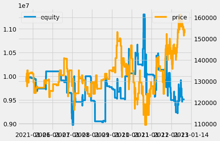
plot_full_equity_curve(data, stats, warmup_bars, lookback_bars)
검증세트로 투자한 것을 연결해서 표현한 그림
                           Equity  DrawdownPct DrawdownDuration
2021-01-05 16:01:00  1.000000e+07      0.00000              NaT
2021-01-05 16:02:00  1.000000e+07      0.00000              NaT
2021-01-05 16:03:00  1.000000e+07      0.00000              NaT
2021-01-05 16:04:00  1.000000e+07      0.00000              NaT
2021-01-05 16:05:00  1.000000e+07      0.00000              NaT
...                           ...          ...              ...
2021-01-13 15:56:00  9.511412e+06      0.08688              NaT
2021-01-13 15:57:00  9.511412e+06      0.08688              NaT
2021-01-13 15:58:00  9.511412e+06      0.08688              NaT
2021-01-13 15:59:00  9.511412e+06      0.08688              NaT
2021-01-13 16:00:00  9.511412e+06      0.08688  0 days 21:41:00

[11520 rows x 3 columns]
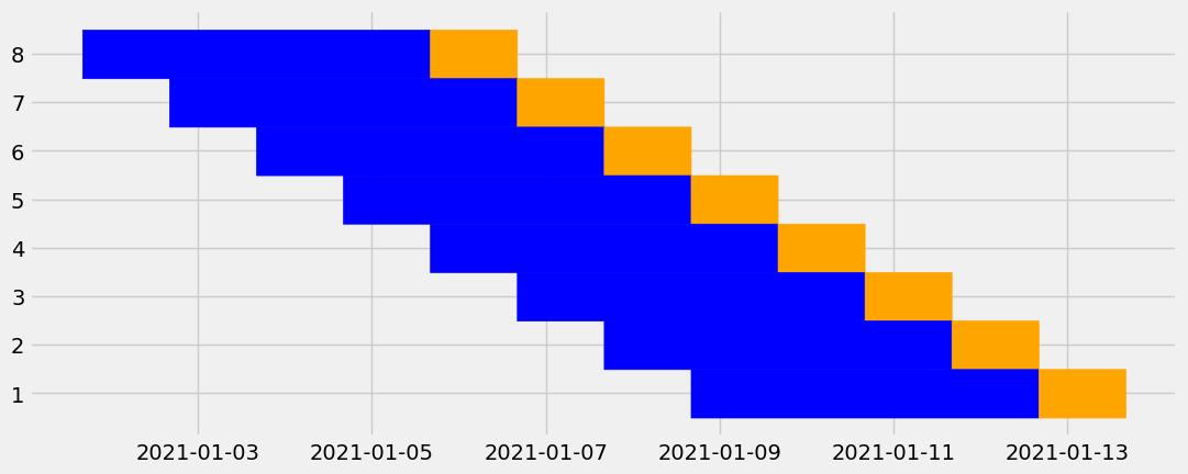
Plot Flow graph of training vs test data
def plot_flow_graph(
    data_full,
    lookback_bars,
    validation_bars):

    ranges = list(range(lookback_bars+warmup_bars, len(data_full) - validation_bars, validation_bars))

    fig, ax = plt.subplots()
    fig.set_figwidth(12)
    for i in range(len(ranges)):
        # 위의 i -> ranges[i]
        # warmup_bars 삭제
        training_data = data_full.iloc[ranges[i]-lookback_bars:ranges[i]]
        validation_data = data_full.iloc[ranges[i]:ranges[i]+validation_bars]

        plt.fill_between(training_data.index,
                         [len(ranges)-i-0.5] * len(training_data.index),
                         [len(ranges)-i+0.5] * len(training_data.index),
                        color='blue')
        plt.fill_between(validation_data.index,
                         [len(ranges)-i-0.5] * len(validation_data.index),
                         [len(ranges)-i+0.5] * len(validation_data.index),
                        color='orange')
    plt.show()
plot_flow_graph(data, lookback_bars, validation_bars)
학습/검증 세트의 구성을 보여주는 그림
8. Fractional Shares in Backtesting.py
https://www.youtube.com/watch?v=3yu4FWmTNh0&list=PLnSVMZC68_e48lA4aRYL1yHYZ9nEq9AiH&index=8&ab_channel=ChadThackray
import datetime
import pandas_ta as ta

from backtesting import Backtest, Strategy
from backtesting.lib import crossover
from backtesting.test import GOOG

print(GOOG)

factor = 1000
GOOG.Open /= factor
GOOG.High /= factor
GOOG.Low /= factor
GOOG.Close /= factor
GOOG.Volume *= factor

print(GOOG)
class RsiOscillator(Strategy):
    upper_bound=70
    lower_bound=30
    rsi_window=14

    def init(self):
        self.rsi = self.I(ta.rsi, self.data.Close.s, self.rsi_window)

    def next(self):
        if crossover(self.rsi, self.upper_bound):
            self.position.close()
        elif crossover(self.lower_bound, self.rsi):
            if not self.position:
                self.buy()

bt = Backtest(GOOG, RsiOscillator, cash=10_000_000, commission=0.002)
stats = bt.run()
display(stats)
bt.plot()
              Open    High     Low   Close    Volume  Signal
2004-08-19  100.00  104.06   95.96  100.34  22351900       1
2004-08-20  101.01  109.08  100.50  108.31  11428600      -1
2004-08-23  110.75  113.48  109.05  109.40   9137200      -1
2004-08-24  111.24  111.60  103.57  104.87   7631300      -1
2004-08-25  104.96  108.00  103.88  106.00   4598900       1
...            ...     ...     ...     ...       ...     ...
2013-02-25  802.30  808.41  790.49  790.77   2303900       1
2013-02-26  795.00  795.95  784.40  790.13   2202500       1
2013-02-27  794.80  804.75  791.11  799.78   2026100      -1
2013-02-28  801.10  806.99  801.03  801.20   2265800      -1
2013-03-01  797.80  807.14  796.15  806.19   2175400       0

[2148 rows x 6 columns]
               Open     High      Low    Close       Volume  Signal
2004-08-19  0.10000  0.10406  0.09596  0.10034  22351900000       1
2004-08-20  0.10101  0.10908  0.10050  0.10831  11428600000      -1
2004-08-23  0.11075  0.11348  0.10905  0.10940   9137200000      -1
2004-08-24  0.11124  0.11160  0.10357  0.10487   7631300000      -1
2004-08-25  0.10496  0.10800  0.10388  0.10600   4598900000       1
...             ...      ...      ...      ...          ...     ...
2013-02-25  0.80230  0.80841  0.79049  0.79077   2303900000       1
2013-02-26  0.79500  0.79595  0.78440  0.79013   2202500000       1
2013-02-27  0.79480  0.80475  0.79111  0.79978   2026100000      -1
2013-02-28  0.80110  0.80699  0.80103  0.80120   2265800000      -1
2013-03-01  0.79780  0.80714  0.79615  0.80619   2175400000       0

[2148 rows x 6 columns]


Start                     2004-08-19 00:00:00
End                       2013-03-01 00:00:00
Duration                   3116 days 00:00:00
Exposure Time [%]                   29.329609
Equity Final [$]              15534282.599116
Equity Peak [$]               15694342.224296
Return [%]                          55.342826
Buy & Hold Return [%]              703.458242
Return (Ann.) [%]                    5.303301
Volatility (Ann.) [%]               23.920019
Sharpe Ratio                          0.22171
Sortino Ratio                        0.371751
Calmar Ratio                         0.107059
Max. Drawdown [%]                   -49.53641
Avg. Drawdown [%]                   -6.240949
Max. Drawdown Duration     1603 days 00:00:00
Avg. Drawdown Duration       94 days 00:00:00
# Trades                                    9
Win Rate [%]                        77.777778
Best Trade [%]                      21.155672
Worst Trade [%]                    -20.607876
Avg. Trade [%]                       5.015784
Max. Trade Duration         202 days 00:00:00
Avg. Trade Duration         101 days 00:00:00
Profit Factor                        3.418112
Expectancy [%]                       5.723001
SQN                                  1.184484
_strategy                       RsiOscillator
_equity_curve                             ...
_trades                          Size  Ent...
dtype: object
stats._trades
| Size | EntryBar | ExitBar | EntryPrice | ExitPrice | PnL | ReturnPct | EntryTime | ExitTime | Duration | |
|---|---|---|---|---|---|---|---|---|---|---|
| 0 | 27572979 | 373 | 422 | 0.362674 | 0.43940 | 2.115567e+06 | 0.211557 | 2006-02-10 | 2006-04-24 | 73 days |
| 1 | 33128895 | 493 | 525 | 0.365710 | 0.41546 | 1.648164e+06 | 0.136037 | 2006-08-03 | 2006-09-19 | 47 days |
| 2 | 24497973 | 862 | 925 | 0.561831 | 0.55794 | -9.533190e+04 | -0.006926 | 2008-01-23 | 2008-04-23 | 91 days |
| 3 | 29227624 | 987 | 1126 | 0.467653 | 0.37128 | -2.816767e+06 | -0.206079 | 2008-07-22 | 2009-02-09 | 202 days |
| 4 | 19813704 | 1367 | 1424 | 0.547683 | 0.56300 | 3.034829e+05 | 0.027967 | 2010-01-25 | 2010-04-16 | 81 days |
| 5 | 22222143 | 1437 | 1534 | 0.501982 | 0.51286 | 2.417334e+05 | 0.021670 | 2010-05-05 | 2010-09-22 | 140 days |
| 6 | 19857019 | 1653 | 1740 | 0.573946 | 0.59249 | 3.682365e+05 | 0.032310 | 2011-03-14 | 2011-07-18 | 126 days |
| 7 | 20527994 | 1873 | 1913 | 0.573124 | 0.64660 | 1.508316e+06 | 0.128203 | 2012-01-26 | 2012-03-23 | 57 days |
| 8 | 20235098 | 2072 | 2129 | 0.655959 | 0.76769 | 2.260882e+06 | 0.170332 | 2012-11-09 | 2013-02-04 | 87 days |
9. Multi-threaded Backtesting in python
멀티스레드를 사용하는 경우 이 예에서는 3배의 속도 차이 발생
#### .py 파일로 실행해야함

# from datetime import datetime
# import pandas_ta as ta
# import pandas as pd
# import os
# import time

# from backtesting import Backtest, Strategy
# from backtesting.lib import crossover

# from multiprocessing import Pool

# class RsiOscillator(Strategy):
#     upper_bound=70
#     lower_bound=30
#     rsi_window=14

#     def init(self):
#         self.rsi = self.I(ta.rsi, self.data.Close.s, self.rsi_window)

#     def next(self):
#         if crossover(self.rsi, self.upper_bound):
#             self.position.close()
#         elif crossover(self.lower_bound, self.rsi):
#             if not self.position:
#                 self.buy()

# def do_backtest(ticker = 'KODEX 200'):
#     start_date = datetime(2018, 1, 1)
#     df = pd.read_pickle("../crawling/data/etf_price.pickle")
#     df.columns = ['NAV','Open','High','Low','Close','Volume','Amount','base','ticker','code','Date']
#     df['Date'] = pd.to_datetime(df['Date'])
#     cond = (df['ticker']==ticker) & (df['Date']>start_date)
#     data = df[cond].reset_index(drop=True)
#     data = data[['Date','Open','High','Low','Close','Volume']].set_index('Date')
#     for col in data.columns:
#         data[col] = pd.to_numeric(data[col]).astype('float')

#     bt = Backtest(data, RsiOscillator, cash=10_000_000, commission=0.002)
#     stats = bt.run()
#     return (ticker, stats['Return [%]'])


# if __name__ == '__main__':
#     tickers = ['KODEX 200선물인버스2X', 'KODEX 미국반도체MV','KODEX 코스피','TIGER 2차전지테마',
#                 'KODEX 미국반도체MV', 'TIGER 200 IT', 'TIGER Fn신재생에너지','TIGER 코스닥150선물인버스',
#                 'KBSTAR 미국S&P원유생산기업(합성 H)']

#     start_time = time.time()
#     with Pool() as p: #after pool is done, this will clean up memory
#         results = p.map(do_backtest, tickers)

#     time_taken = time.time() - start_time
#     print(f"Took {time_taken} seconds")
#     print(results)
from datetime import datetime
import pandas_ta as ta
import pandas as pd
import os
import time

class RsiOscillator(Strategy):
    upper_bound=70
    lower_bound=30
    rsi_window=14

    def init(self):
        self.rsi = self.I(ta.rsi, self.data.Close.s, self.rsi_window)

    def next(self):
        if crossover(self.rsi, self.upper_bound):
            self.position.close()
        elif crossover(self.lower_bound, self.rsi):
            if not self.position:
                self.buy()

def do_backtest(ticker = 'KODEX 200'):
    start_date = datetime(2018, 1, 1)
    df = pd.read_pickle("../crawling/data/etf_price.pickle")
    df.columns = ['NAV','Open','High','Low','Close','Volume','Amount','base','ticker','code','Date']
    df['Date'] = pd.to_datetime(df['Date'])
    cond = (df['ticker']==ticker) & (df['Date']>start_date)
    data = df[cond].reset_index(drop=True)
    data = data[['Date','Open','High','Low','Close','Volume']].set_index('Date')
    for col in data.columns:
        data[col] = pd.to_numeric(data[col]).astype('float')

    bt = Backtest(data, RsiOscillator, cash=10_000_000, commission=0.002)
    stats = bt.run()
    return (ticker, stats['Return [%]'])

tickers = ['KODEX 200선물인버스2X', 'KODEX 미국반도체MV','KODEX 코스피','TIGER 2차전지테마',
            'KODEX 미국반도체MV', 'TIGER 200 IT', 'TIGER Fn신재생에너지','TIGER 코스닥150선물인버스',
            'KBSTAR 미국S&P원유생산기업(합성 H)']
tickers = tickers*10
start_time = time.time()
for ticker in tickers:
    print(do_backtest(ticker))

time_taken = time.time() - start_time
print(f"Took {time_taken} seconds")
('KODEX 200선물인버스2X', -58.9937544)
('KODEX 미국반도체MV', 18.611619400000013)
('KODEX 코스피', -26.63166719999997)
('TIGER 2차전지테마', 126.3208749)
('KODEX 미국반도체MV', 18.611619400000013)
('TIGER 200 IT', 13.659680999999976)
('TIGER Fn신재생에너지', 9.86832450000001)
('TIGER 코스닥150선물인버스', 34.32884810000002)
('KBSTAR 미국S&P원유생산기업(합성 H)', -20.03688280000001)
Took 19.13048505783081 seconds
댓글남기기